Applications¶

Once a sGDML model is trained (see force field reconstruction), it can be used like any other force field. Here, we show a few typical applications. Additional practical examples can be found in Chmiela et al. 2019 1.

1: Chmiela, S., Sauceda, H. E., Poltavsky, Igor, Müller, K.-R., Tkatchenko, A. (2019). sGDML: Constructing Accurate and Data Efficient Molecular Force Fields Using Machine Learning. ‎Comput. Phys. Commun., 240, 38-45.

Warning

The examples below rely on tools from the Atomic Simulation Environment (ASE), which expects eV and Angstrom as energy and length units, respectively. However, sGDML models are unit agnostic, which is why a unit conversion might be necessary.

By default, the included SGDMLCalculator ASE interface assumes that kcal/mol and Angstrom are used in the model and performs the appropriate conversion. Please specify your own conversion factors via the keyword arguments E_to_eV and F_to_eV_Ang during initialization, if your model uses different units.

E_to_eV specifies the factor from the energy unit used in the model to eV.

F_to_eV_Ang specifies factor from the force unit used in the model to eV/Ang.

MD simulations¶

The following example (based on this tutorial) shows how to run a constant-energy molecular dynamics (MD) simulation of ethanol at a temperature of 300 K and a resolution of 0.2 fs for 100 ps. A pre-trained ethanol model can be downloaded as described here. As starting point, a geometry file ethanol.xyz in XYZ format is also needed (download).

from sgdml.intf.ase_calc import SGDMLCalculator

from ase.io import read
from ase.optimize import QuasiNewton
from ase.md.velocitydistribution import (MaxwellBoltzmannDistribution, Stationary, ZeroRotation)
from ase.md.verlet import VelocityVerlet
from ase import units

model_path = 'm_ethanol.npz'
calc = SGDMLCalculator(model_path)

mol = read('ethanol.xyz')
mol.set_calculator(calc)

# do a quick geometry relaxation
qn = QuasiNewton(mol)
qn.run(1e-4, 100)

# set the momenta corresponding to T=300K
MaxwellBoltzmannDistribution(mol, 300 * units.kB)
Stationary(mol) # zero linear momentum
ZeroRotation(mol) # zero angular momentum

# run MD with constant energy using the velocity verlet algorithm
dyn = VelocityVerlet(mol, 0.2 * units.fs, trajectory='md.traj')  # 0.2 fs time step.

def printenergy(a):
        # function to print the potential, kinetic and total energy
        epot = a.get_potential_energy() / len(a)
        ekin = a.get_kinetic_energy() / len(a)
        print('Energy per atom: Epot = %.3feV  Ekin = %.3feV (T=%3.0fK)  '
                'Etot = %.3feV' % (epot, ekin, ekin / (1.5 * units.kB), epot + ekin))

# now run the dynamics
printenergy(mol)
for i in range(10000):
        dyn.run(10)
        printenergy(mol)

Visualizing results¶

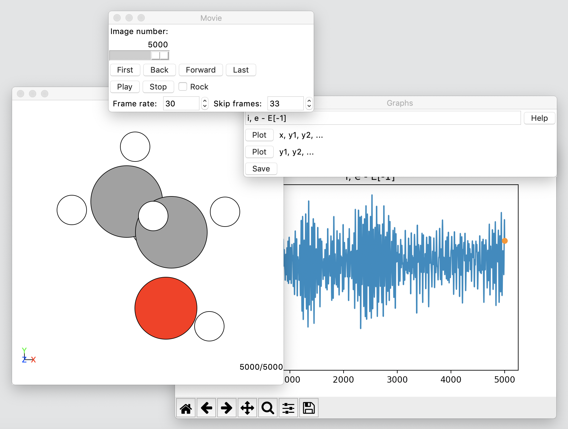
The code above first relaxes the given geometry in the provided force field model, before running an MD simulation. It will then output a trajectory file md.traj that can be visualized by running

$ ase gui md.traj

The result will look something like this:

You can easily export each step of this trajectory as individual Extended XYZ files using the following code snippet:

import sys
import os.path
from ase.io.trajectory import Trajectory
from ase.io import write

our_dir = 'out'
if os.path.isdir(our_dir):
        sys.exit('Output directory already exists.')
else:
        os.mkdir(our_dir)

traj = Trajectory('md.traj')
for i,atoms in enumerate(traj):
        atoms.wrap()
        write(our_dir + '/step'+("{:05d}".format(i))+'.xyz', atoms, append=False)

Vibrational modes¶

The following example (based the tutorial here) shows how to obtain the vibrational modes for ethanol. Once again, a pre-trained model ethanol.npz and a geometry file ethanol.xyz in XYZ format (download) are needed.

from sgdml.intf.ase_calc import SGDMLCalculator

from ase.io import read
from ase.optimize import QuasiNewton
from ase.vibrations import Vibrations

model_path = 'ethanol.npz'
calc = SGDMLCalculator(model_path)

mol = read('ethanol.xyz')
mol.set_calculator(calc)

# do a quick geometry relaxation
qn = QuasiNewton(mol)
qn.run(1e-4, 100)

# run the vibration calculations
vib = Vibrations(mol)
vib.run()

vib.summary() # print a summary of the vibrational frequencies
vib.write_jmol() # write file for viewing of the modes with jmol

vib.clean() # remove pickle-files

The result will look something like this:

---------------------
  #    meV     cm^-1
---------------------
  1.4i     11.1i
  0.5i      4.1i
  0.1i      0.9i
  0.0i      0.0i
  0.0       0.4
  0.1       0.9
 27.6     222.8
 33.8     273.0
 50.2     405.0
 97.9     789.9
108.0     870.7
124.0    1000.3
133.1    1073.9
141.0    1137.5
153.4    1237.6
155.8    1256.7
166.6    1344.0
173.5    1399.0
177.7    1433.0
180.2    1453.8
181.8    1466.6
358.9    2894.5
364.9    2943.4
368.4    2971.1
377.9    3047.8
379.0    3056.6
461.2    3719.5
---------------------
Zero-point energy: 2.108 eV

Note

Imaginary frequencies indicate that the geometry is not yet perfectly relaxed.

Visualizing results¶

The code above also outputs a file vib.xyz that can be used to visualize the modes, e.g. using Jmol. Here is vibrational mode #8 from the previous table:

Vibrational spectra¶

Vibrational modes only provide the vibrational spectrum of a system within the harmonic approximation, i.e. the potential energy surface is assumed to behave like a harmonic potential centered at a local minimum. To get a more complete picture, we can look at the power spectrum of the autocorrelation of the nuclear velocities, where many anharmonic effects become visible. While all frequency peaks have the same intensity in a harmonic approximation, anharmonicity causes a broadening of the bands, which influences the intensities.

The following example shows how to use the MD trajectory generated in the MD simulations section. We reuse the nuclear velocities from the trajectory file md.traj (download) that were generated during the MD simulations already.

import numpy as np
from scipy.fftpack import fft, fftfreq
from ase.io.trajectory import Trajectory

def pdos(V, dt):
    """
    Calculate the phonon density of states from a trajectory of
    velocities (power spectrum of the velocity auto-correlation
    function).

    Parameters
    ----------
    V : :obj:`numpy.ndarray`
        (dims N x T) velocities of N degrees of freedom for
        trajetory of length T
    dt : float
        time between steps in trajectory (fs)

    Returns
    -------
    freq : :obj:`numpy.ndarray`
        (dims T) Frequencies (cm^-1)
    pdos : :obj:`numpy.ndarray`
        (dims T) Density of states (a.u.)
    """

    n_steps = V.shape[1]

    # mean velocity auto-correlation for all degrees of freedom
    vac2 = [np.correlate(v, v, 'full') for v in V]
    vac2 /= np.linalg.norm(vac2, axis=1)[:, None]
    vac2 = np.mean(vac2, axis=0)

    # power spectrum (phonon density of states)
    pdos = np.abs(fft(vac2))**2
    pdos /= np.linalg.norm(pdos) / 2 # spectrum is symmetric

    freq = fftfreq(2*n_steps-1, dt) * 33356.4095198152 # Frequency in cm^-1

    return freq[:n_steps], pdos[:n_steps]

# load MD trajectory
traj = Trajectory('md.traj')

# read velocities
V = np.array([atoms.get_velocities() for atoms in traj])

# time step that was used for the MD simulation
dt = 0.2

n_steps = V.shape[0]
V = V.reshape(n_steps, -1).T
freq, pdos = pdos(V, dt)

# smoothing of the spectrum
# (removes numerical artifacts due to finite time trunction of the FFT)
from scipy.ndimage.filters import  gaussian_filter1d as gaussian
pdos = gaussian(pdos, sigma=50)

Note

The auto-correlation is calculated for each of the 3N degrees of freedom of the molecule and the sum of all correlation functions is Fourier transformed to get the power spectrum of that molecule.

Visualizing results¶

import matplotlib.pyplot as plt

plt.plot(freq, pdos)
plt.yticks([])
plt.xlim(0, 4000)

plt.box(on=None)

plt.xlabel('Frequency [cm$^{-1}$]')
plt.ylabel('Density of states [a.u.]')
plt.title('Velocity auto-correlation function\n(ethanol 300K, 0.2 fs)')
plt.savefig('vaf.png')
plt.show()

The code above generates a figure vaf.png that looks something like this:

Minima hopping¶

The next example (based on this tutorial) shows how to search for a globally optimal geometric configuration using the minima hopping algorithm. Once again, a pre-trained ethanol model ethanol.npz and a geometry file ethanol.xyz in XYZ format (download) are the starting point:

from sgdml.intf.ase_calc import SGDMLCalculator

from ase.io import read
from ase.optimize import QuasiNewton
from ase.optimize.minimahopping import (MinimaHopping, MHPlot)

model_path = 'ethanol.npz'
calc = SGDMLCalculator(model_path)

mol = read('ethanol.xyz')
mol.set_calculator(calc)

# do a quick geometry relaxation
qn = QuasiNewton(mol)
qn.run(1e-4, 100)

# instantiate and run the minima hopping algorithm
hop = MinimaHopping(mol, T0=4000., fmax=1e-4)
hop(totalsteps=5)

plot = MHPlot()
plot.save_figure('ase_mh.png')

Visualizing results¶

The script above will run five molecular dynamics trajectories, each generating its own output file. It will also produce a file called minima.traj which contains all accepted minima. Those can be easily viewed with ASE, using:

$ ase gui minima.traj

We can also easily convert it to other formats, such as Extended XYZ:

$ ase convert minima.traj minima.xyz

This command renders the first found minimum as PNG file:

$ ase convert -n 0 minima.traj minimum_0.png

Here are renderings of the structures found in each of the five runs (some minimas are visited multiple times):

Additionally, the minima hopping process is visualized in a summary figure ase_mh.png. As the search is inherently random, your results will look different. In this example, the two distinct minima of ethanol have been successfully found:

This type of plot is described here:

“In this figure, you will see on the \(E_{\text{pot}}\) axes the energy levels of the conformers found. The flat bars represent the energy at the end of each local optimization step. The checkmark indicates the local minimum was accepted; red arrows indicate it was rejected for the three possible reasons. The black path between steps is the potential energy during the MD portion of the step; the dashed line is the local optimization on termination of the MD step. Note the y axis is broken to allow different energy scales between the local minima and the space explored in the MD simulations. The \(T\) and \(E_{\text{diff}}\) plots show the values of the self-adjusting parameters as the algorithm progresses.”